Linear Regression From Scratch

Linear Regression is a type of model which assumes linear relationship between input variables and target variables. It is used to calculate or predict a value based on one(or many) input variables. It is generally used when:

• You have a linear relationship ,suppose x and y are two variables and they have a direct (one increases , other also increases) or an indirect (one increases, other decreases) relationship.
• When you have to predict a numerical value, in case you have categorical values you have to convert it into numerical for performing a linear regression model.
• You have one dependent and one independent variable.

Best-Fit line

Linear Regression model is straight line which best fits the data. Its equation is:

Where:

1. m is the slope or the gradient of the line
2. c is the y-intercept of the line

Multiple Linear Regression (MLR) is used when there are more than one input variables. In this article I’ll be implementing a Linear Regression model for a single input variable from scratch in python using numpy and matplotlib and explaining the idea behind each step(with the full code at the end).

Getting Started

1. Numpy is a python library which is used for calculating high level mathematical operations on large multi-dimensional arrays and matrices.
2. Matplotlib is a graphing library which will help in plotting various graphs to make data interpretation easy.
3. Math module has some built-in functions like square root which will help in calculating values.

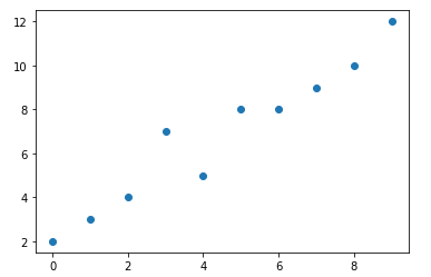
Now , Here I am defining two arrays , one is input or independent variable (x) and the other is output or dependent variable (y) and inserting some values into both of them and then plotting the resulting points on a graph.

ScatterPlot

Defining Terms and Calculating Values

Mean: It is the sum of observations divided by the count of observations.

Output

Variance: It is a measure of how far the observations are from the mean.

Standard Deviation: It is the measure of amount of variance.

Standard Deviation is denoted by σ (sigma) , which is the square root of variance.

Standard Deviation (unbiased)

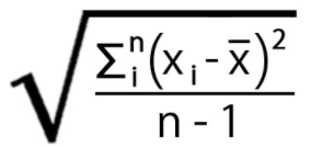
Where :

1. xᵢ is the observation
2. x̅ is the mean
3. n is the total number of observations.

Output

Note: In calculating variance/standard deviation , we have divided by n-1 instead of n , this is to ensure the variance/standard deviation is unbiased. Look into Bessel’s correction for more information.

Sum of Squares: Is used to identify the dispersion of data, it is the sum of squares of the difference between all the points and the mean.

Sum Of Squares

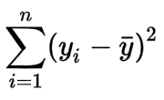
Where:

1. yᵢ is the observation
2. y̅ is the mean
3. n is the number of observations

Output

Deviation Score: It is the summation of difference between all the observations and the mean of the observations.

Product of Deviation Scores

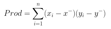
Where:

1. xᵢ, yᵢ is the observation
2. x⁻, y⁻ is the mean of x and y respectively
3. n is the number of observations

Output

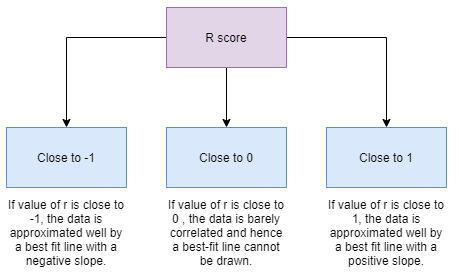
R score: It is the correlation between the predicted and actual values. Its value ranges from -1 to +1.

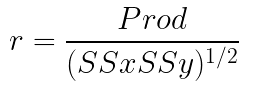
Where:

1. Prod is the product of deviation scores
2. SSx is the sum of squares for X
3. SSy is the sum of squares for Y

Output

Slope: It is a measure of how steep a straight line is.

Which is calculated by:

Where:

1. m is the slope.
2. stdev is the standard deviation.
3. r is the r score.

Output

Result

Now that we’ve obtained the slope, we can write the equation of best-fit line as:

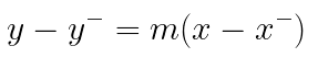
Where y⁻ and x⁻ is the mean of y and x respectively and m is the slope.

Output

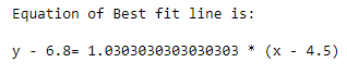
Now plotting the best fit line on top of the scatter plot.

Best-Fit line

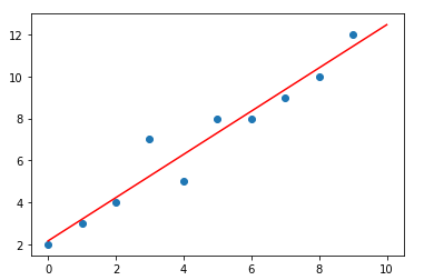
This is the best-fit line which we’ve obtained for the given arrays x and y , It can now be used to predict future values.

Verification

Now using sklearn to verify whether our best-fit line is correct or not.

Reshaping the arrays so that they can be used in the LinearRegression() function. Reshaping changes the shape of the array without changing the content.

Output

Conclusion

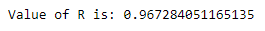
The value of r obtained is 0.9672 and the value of r obtained from using sklearn is 0.9672 , since they’re both the same , we have arrived at the same best-fit line but without using any of the machine learning libraries. This approach is purely statistical and can be used to predict or for regression analysis.

Full Code